Prokaryotic Genome GC Content
Visualizing the distribution of prokaryotic genome GC content within phyla.
Introduction
Prokaryotic genomes vary in GC content. Indeed, the percent GC content of a prokaryotic genome is considered a characteristic of the organism, and closely-related organisms often have similar GC contents. Even at the phylum level of the taxnomic hierarchy for prokaryotes, organisms may share a similar range of GC contents. For example, Actinobacteria are sometimes referred to as the high GC gram positives while Firmicutes are referred to as the low GC gram positives. In this blogpost, I will use the same data table of 11,710 RefSeq representative prokaryotic genomes that was used in a prior blogpost where I examined genome size, except I will analyze the column indicating the percent GC content of the genome.
Load libraries
Let’s load all the required libraries upfront so that one doesn’t have to search each code snippet for the required packages.
library(ggplot2)
library(tidyverse)
## ── Attaching packages ───────────────────────────────────────────────────────────────────────────────────────────────────────── tidyverse 1.3.0 ──## ✔ tibble 2.1.3 ✔ dplyr 0.8.3
## ✔ tidyr 1.0.0 ✔ stringr 1.4.0
## ✔ readr 1.3.1 ✔ forcats 0.4.0
## ✔ purrr 0.3.3## ── Conflicts ──────────────────────────────────────────────────────────────────────────────────────────────────────────── tidyverse_conflicts() ──
## ✖ dplyr::filter() masks stats::filter()
## ✖ dplyr::lag() masks stats::lag()Load the Data and Produce Summary Statistics
I will begin by loading the aforementioned table of prokaryotic genome metadata, and then I will geneate summary data to examine the range of GC contents for the prokaryotes represented in that table.
setwd("/home/chrisgaby/github/My_Website/")

# Read the table into a tibble.
prokaryote.genomes.table <- read_csv(file = "./static/files/prokaryotes.csv")

# Display the minimum, maximum, mean, median, and 1st and 3rd quartiles
# for the genome sizes.
summary(prokaryote.genomes.table$`GC%`)
## Min. 1st Qu. Median Mean 3rd Qu. Max.
## 22.40 41.00 54.80 53.18 65.50 77.00It looks like GC% ranges from 22.4 to 77%, a difference of 54.6%!
Histogram of GC%
Let’s examine the distribution of GC% for all the prokaryotic genomes.
qplot(data = prokaryote.genomes.table,
      x = `GC%`,
      binwidth = 1)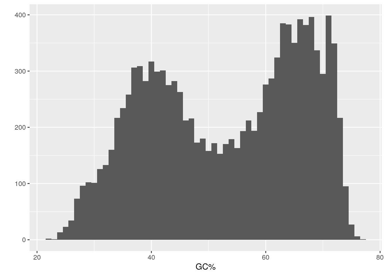
The distribution is bimodal.
GC% for the Principle Taxonomic Groupings
Note that the descriptors used in the table to refer to taxonomy include multi-phylum groupings like “FCB group”, “PVC group”, and “Terrabacteria”. Hence, we’ll separate the “Organism Groups” column with this information into 3 new columns for the taxonomic levels (TL) designated TL1, TL2, and TL3, and then we’ll examine the GC% distribution for the 6 most abundant groups at TL2.
# Split the Organism Groups column into new columns named according to their
# respective taxonomy level, abbreviated TL1, TL2, and TL3.
prokaryote.genomes.table.split <- separate(data=prokaryote.genomes.table,
                                           col = `Organism Groups`,
                                           sep = ";",
                                           into = c("TL1", "TL2", "TL3"))

TL2.subset.names <- names(which(summary(factor(prokaryote.genomes.table.split$TL2)) > 90))
prokaryote.genomes.table.split.reduced <- prokaryote.genomes.table.split[prokaryote.genomes.table.split$TL2 == TL2.subset.names[1] |
                                 prokaryote.genomes.table.split$TL2 == TL2.subset.names[2] |
                                 prokaryote.genomes.table.split$TL2 == TL2.subset.names[3] |
                                 prokaryote.genomes.table.split$TL2 == TL2.subset.names[4] |
                                 prokaryote.genomes.table.split$TL2 == TL2.subset.names[5] |
                                 prokaryote.genomes.table.split$TL2 == TL2.subset.names[6],]

qplot(data=prokaryote.genomes.table.split.reduced,
      x = `GC%`,
      geom = "density",
      color = TL2,
      fill = TL2,
      alpha = I(0.2))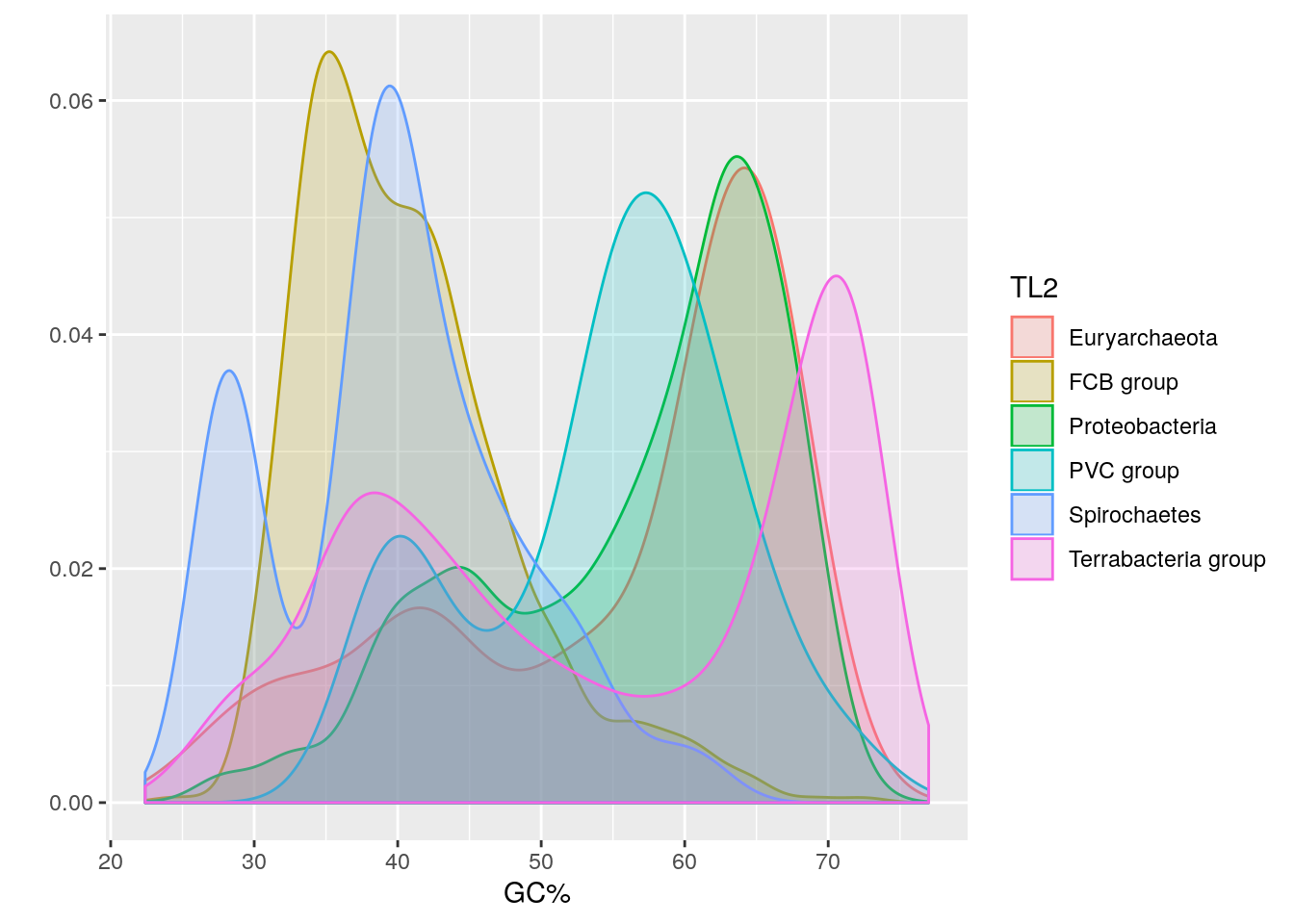
It looks like some phyla have a bimodal GC% distribution too.
Faceted Phylum GC%
Let’s separate these TL2 groups into their own facets.
qplot(data=prokaryote.genomes.table.split.reduced,
      x = `GC%`,
      geom = "density",
      color = TL2,
      fill = TL2,
      facets = TL2 ~ .)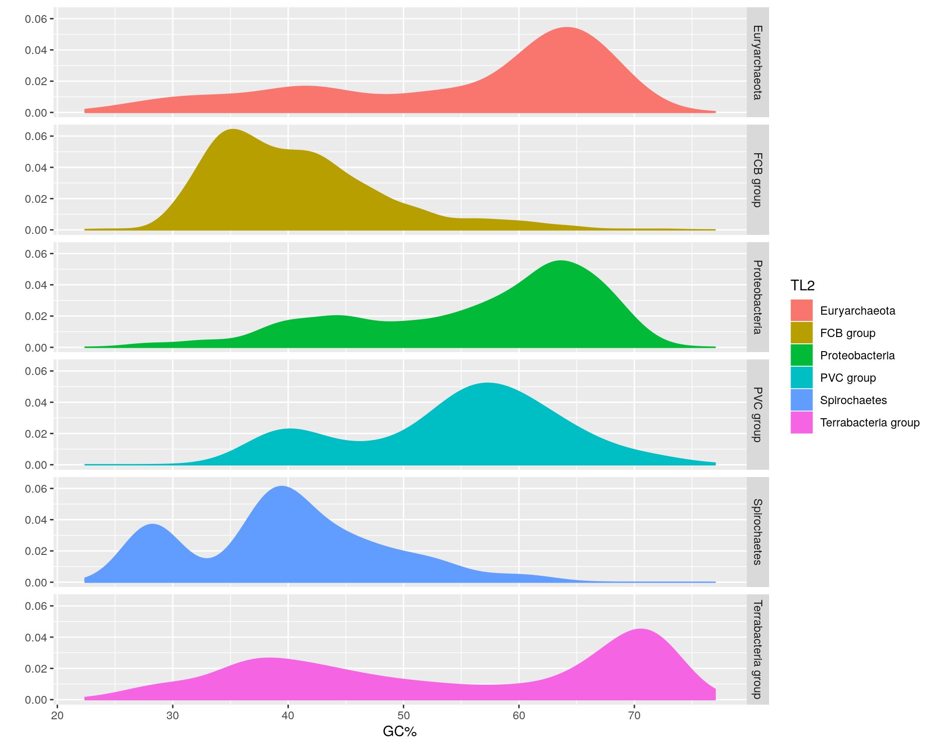
The Proteobacteria and Spirochaetes have bimodal genome GC% distributions, and thus it seems there are taxa within these phyla with distinct GC% contents.
Some of these designations like PVC group and Terrabacteria group are supercategories that contain several traditional phyla.
Terrabacteria Phyla GC%
Let’s divide the Terrabacteria group up into the phyla that comprise it.
# Display the taxa within Terrabacteria.
unique(prokaryote.genomes.table.split[prokaryote.genomes.table.split$TL2 ==
                                        "Terrabacteria group","TL3"])
## # A tibble: 9 x 1
## TL3
## <chr>
## 1 Firmicutes
## 2 Actinobacteria
## 3 Cyanobacteria/Melainabacteria group
## 4 Tenericutes
## 5 Deinococcus-Thermus
## 6 Chloroflexi
## 7 unclassified Terrabacteria group
## 8 Armatimonadetes
## 9 AbditibacteriotaThe Terrabacteria group contains both the high and low GC gram positives Actinobacteria and Firmicutes. Let’s see if we have enough data points in each phylum to create another distribution.
# The number of rows for each phylum indicates the number of datapoints
# for each phylum
nrow(prokaryote.genomes.table.split[prokaryote.genomes.table.split$TL3 ==
                                      "Actinobacteria",])
## [1] 2319nrow(prokaryote.genomes.table.split[prokaryote.genomes.table.split$TL3 ==
"Firmicutes",])## [1] 2217nrow(prokaryote.genomes.table.split[prokaryote.genomes.table.split$TL3 ==
"Cyanobacteria/Melainabacteria group",])## [1] 134nrow(prokaryote.genomes.table.split[prokaryote.genomes.table.split$TL3 ==
"Tenericutes",])## [1] 159nrow(prokaryote.genomes.table.split[prokaryote.genomes.table.split$TL3 ==
"Deinococcus-Thermus",])## [1] 73nrow(prokaryote.genomes.table.split[prokaryote.genomes.table.split$TL3 ==
"Chloroflexi",])## [1] 43nrow(prokaryote.genomes.table.split[prokaryote.genomes.table.split$TL3 ==
"unclassified Terrabacteria group",])## [1] 1nrow(prokaryote.genomes.table.split[prokaryote.genomes.table.split$TL3 ==
"Armatimonadetes",])## [1] 3nrow(prokaryote.genomes.table.split[prokaryote.genomes.table.split$TL3 ==
"Abditibacteriota",])## [1] 1It looks like only Actinobacteria, Firmicutes, Cyanobacteria/Melainabacteria group, and Tenericutes have more than 100 data points. We’ll proceed with these 4 phyla for the following visualization.
# Create a Terrabacteria dataframe with only the 4 phyla haveing over 100 datapoints.
Terra.4TL2.df <- prokaryote.genomes.table.split[prokaryote.genomes.table.split$TL3 == "Actinobacteria" |
  prokaryote.genomes.table.split$TL3 == "Firmicutes" |
  prokaryote.genomes.table.split$TL3 == "Cyanobacteria/Melainabacteria group" |
  prokaryote.genomes.table.split$TL3 == "Tenericutes",]

# Create the plot faceted by the information in the TL3 column.
qplot(data=Terra.4TL2.df,
      x = `GC%`,
      geom = "density",
      color = TL3,
      fill = TL3,
      facets = TL3 ~ .)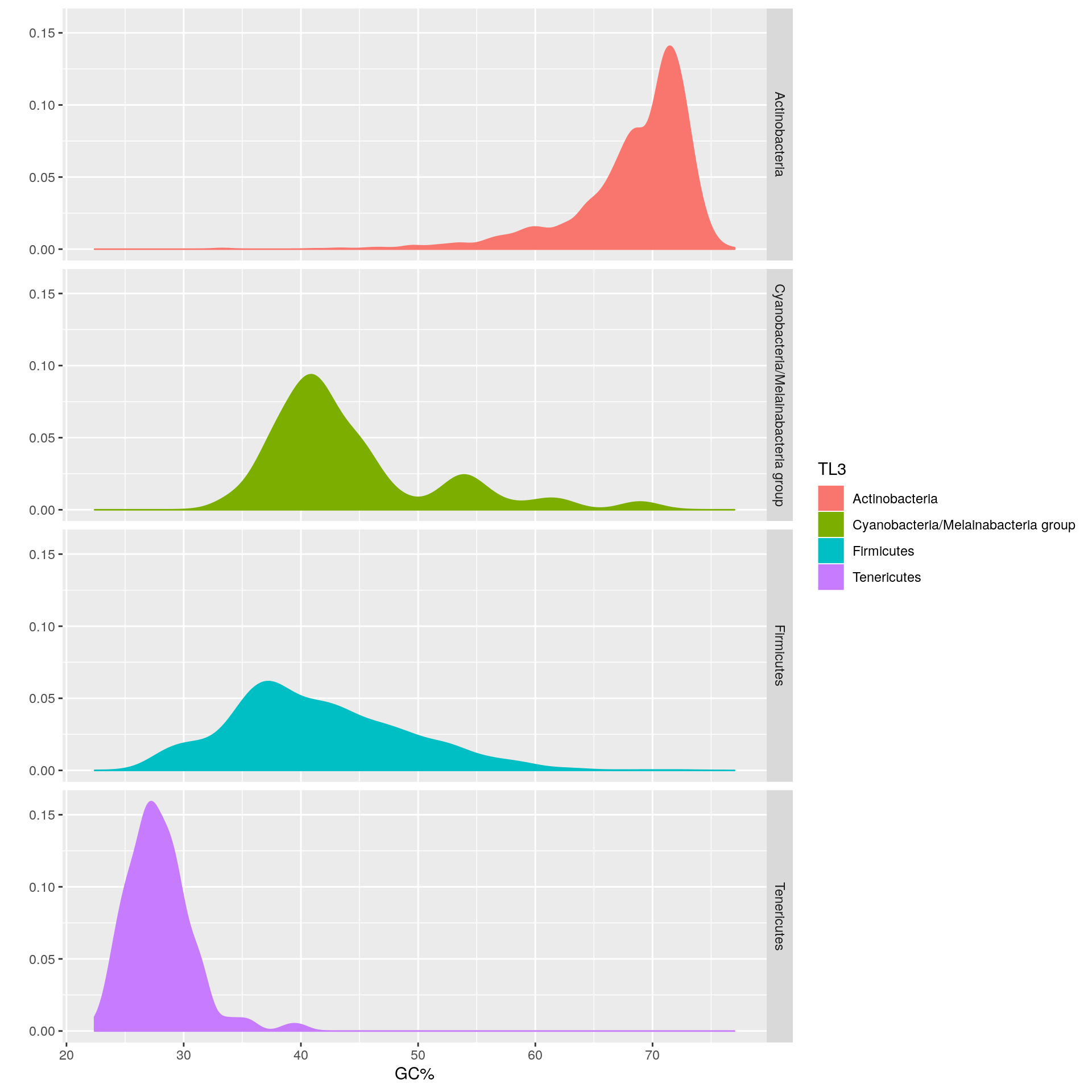
The Firmicutes have a median GC% of 40.3% vs. the Actinobacteria whose median GC% is 69.9%.
The Firmicutes exhibit a wide distribution of genome GC%, thereby leading to a standard deviation of 7.3900331, whereas the Tenericutes have a relatively narrow distribution, with a corresponding standard deviation of 2.7652308.
Conclusion
Genome GC content can vary by more than 50% depending on the organism. Closely-related organisms tend to have similar GC%. For example, Actinobacteria are high GC%, gram positive organisms whose median GC% was determined to be 70% herein, while the Firmicutes are low GC%, gram postitive organisms whose median GC% was 40% herein. Based upon the current genome representation in this dataset, some phyla like the the Tenericutes have a narrow distribution of GC% whereas others like the Firmicutes have a wide range. Still other phyla like the Proteobacteria and Spirochaetes appear bimodal, suggesting that there are lower order taxa in these phyla with distinct genome GC% contents.