Prokaryotic Genome Size
Calculation of summary statistics based upon the 11,710 RefSeq representative prokaryotic genomes
Introduction
Prokaryotic genomes encompass a range of sizes whereby larger genomes may encode more genes that allow for the organism to respond to their environment and smaller, streamlined genomes may indicate adaptation to a less varying, host environment. I will use the table of RefSeq representative genomes downloaded from the NCBI Prokaryotic Genomes page to derive summary statistics and figures that describe the distribution of prokaryotic genome sizes.
The Size of a Prokaryotic Genomes
As a frame of reference, the familiar laboratory workhorse Escherichia coli K12 has a genome size of 4.64 Mb.
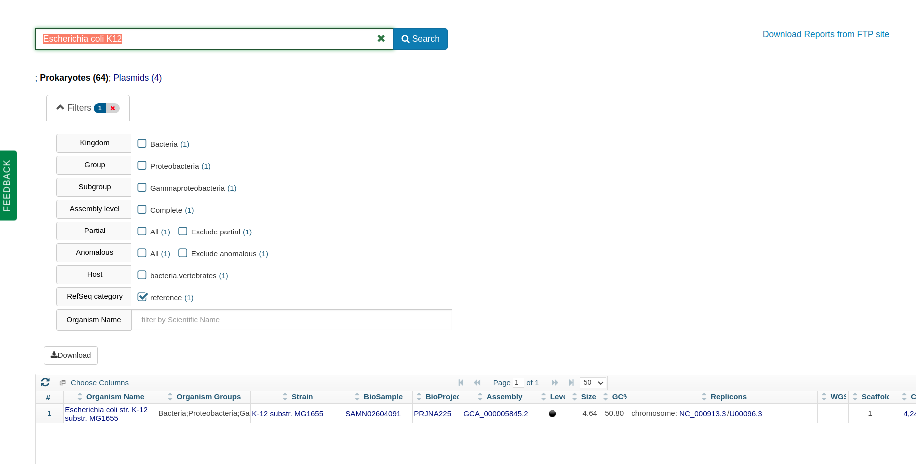
The E coli K12 reference genome from NCBI prokaryotic genomes.
On August 31, 2020, I downloaded a list of the NCBI RefSeq Prokaryotic Genomes. The list included statistics such as genome length for each genome.
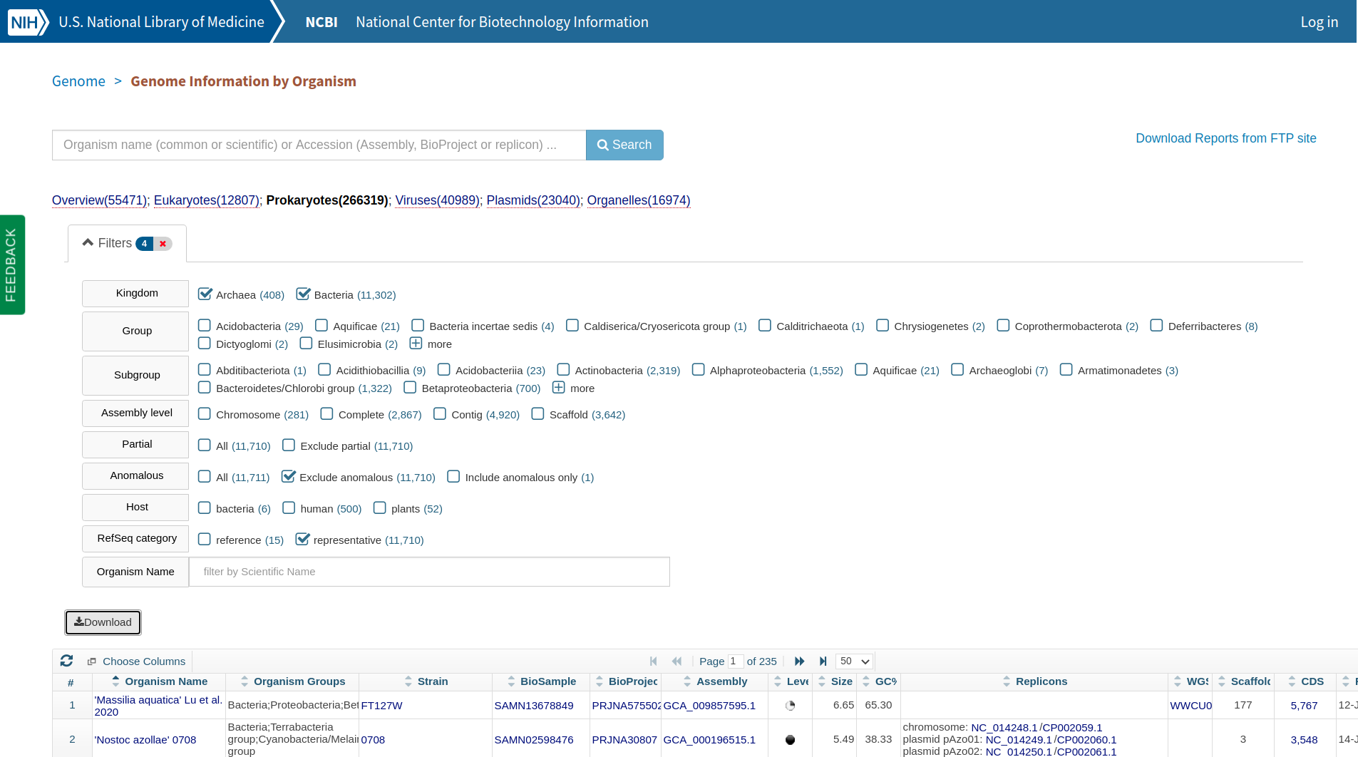
The Criteria Selected to Obtain a List of NCBI Refseq Prokaryotic Genomes.
The list was downloaded from NCBI as a csv file, and I have made this file available for download. Let’s import the csv file and calculate some statistics for prokaryotic genome size.
library(tidyverse)

# Read the table into a tibble.
prokaryote.genomes.table <- read_csv(file = "prokaryotes.csv")

# Display the first few lines of the data frame.
head(prokaryote.genomes.table)
## # A tibble: 6 x 16
## `#Organism Name` `Organism Group… Strain BioSample BioProject Assembly Level
## <chr> <chr> <chr> <chr> <chr> <chr> <chr>
## 1 Pseudomonas flu… Bacteria;Proteo… DR397 SAMN1397… PRJNA6044… GCA_010… Comp…
## 2 Xanthomonas cam… Bacteria;Proteo… MAFF1… SAMN1534… PRJNA6412… GCA_013… Comp…
## 3 Yersinia pestis… Bacteria;Proteo… A1122 SAMN0260… PRJNA67155 GCA_000… Comp…
## 4 Staphylococcus … Bacteria;Terrab… ATCC … SAMN1073… PRJNA5153… GCA_006… Comp…
## 5 Lactococcus lac… Bacteria;Terrab… WFLU12 SAMN0821… PRJNA4231… GCA_002… Cont…
## 6 Bacillus cereus Bacteria;Terrab… FDAAR… SAMN1105… PRJNA2312… GCA_013… Comp…
## # … with 9 more variables: `Size(Mb)` <dbl>, `GC%` <dbl>, Replicons <chr>,
## # WGS <chr>, Scaffolds <dbl>, CDS <dbl>, `Release Date` <dttm>, `GenBank
## # FTP` <chr>, `RefSeq FTP` <chr># How many genomes have data for length?
length(prokaryote.genomes.table$`Size(Mb)`)## [1] 11710# Display the minimum, maximum, mean, median, and 1st and 3rd quartiles for the genome sizes.
summary(prokaryote.genomes.table$`Size(Mb)`)## Min. 1st Qu. Median Mean 3rd Qu. Max.
## 0.185 2.992 4.051 4.372 5.279 16.041Let’s look at the summary statistics for genome size:
- n = 11710
- mean = 4.371931
- minimum = 0.185014
- maximum = 16.0407
- median = 4.050955
There is well over an order of magnitude variation in the size of prokaryotic genomes, ranging from 0.185014 to 16.0407. The largest genome among the refseq genomes belongs to Minicystis rosea whereas the smallest genome belongs to Metaprevotella massiliensis. It is notable that the smallest genome is classified as a Scaffold and thus may not be accurate.
Let’s also take a look at the distribution:
library(ggplot2)

qplot(data = prokaryote.genomes.table,
      x = `Size(Mb)`,
      binwidth = 1)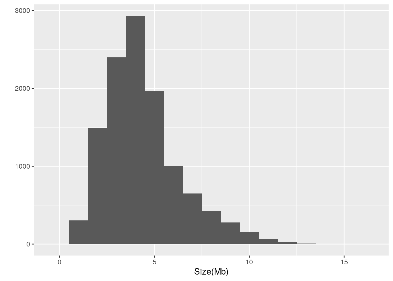
Let’s see how many genomes are available for each phylum in this dataset:
library(tidyr)

# Split the Organism Groups column into new columns named according to their respective taxonomy level
prokaryote.genomes.table.split <- separate(data=prokaryote.genomes.table,
                                           col = `Organism Groups`,
                                           sep = ";",
                                           into = c("Domain", "Phylum", "Class"))

summary(factor(prokaryote.genomes.table.split$Phylum))
## Acidobacteria Aquificae
## 29 21
## Bacteria incertae sedis Caldiserica/Cryosericota group
## 4 1
## Calditrichaeota Chrysiogenetes
## 1 2
## Coprothermobacterota Deferribacteres
## 2 8
## Dictyoglomi Elusimicrobia
## 2 2
## Euryarchaeota FCB group
## 346 1329
## Fusobacteria Nitrospinae/Tectomicrobia group
## 38 1
## Nitrospirae Proteobacteria
## 10 4592
## PVC group Spirochaetes
## 98 141
## Synergistetes TACK group
## 19 62
## Terrabacteria group Thermodesulfobacteria
## 4950 12
## Thermotogae
## 40It looks like there are only a few phyla that have enough genomes to make a reliable histogram, so lets create a new dataset with only those phyla having > 90 genomes.
Let’s break the distribution down into separate density plots for each of the 6 phyla with over 90 genomes:
library(ggplot2)

phyla.subset.names <- names(which(summary(factor(prokaryote.genomes.table.split$Phylum)) > 90))
prokaryote.genomes.table.split.reduced <- prokaryote.genomes.table.split[prokaryote.genomes.table.split$Phylum == phyla.subset.names[1] |
                                 prokaryote.genomes.table.split$Phylum == phyla.subset.names[2] |
                                 prokaryote.genomes.table.split$Phylum == phyla.subset.names[3] |
                                 prokaryote.genomes.table.split$Phylum == phyla.subset.names[4] |
                                 prokaryote.genomes.table.split$Phylum == phyla.subset.names[5] |
                                 prokaryote.genomes.table.split$Phylum == phyla.subset.names[6],]

qplot(data=prokaryote.genomes.table.split.reduced,
      x = `Size(Mb)`,
      geom = "density",
      color = Phylum,
      fill = Phylum,
      alpha = I(0.2))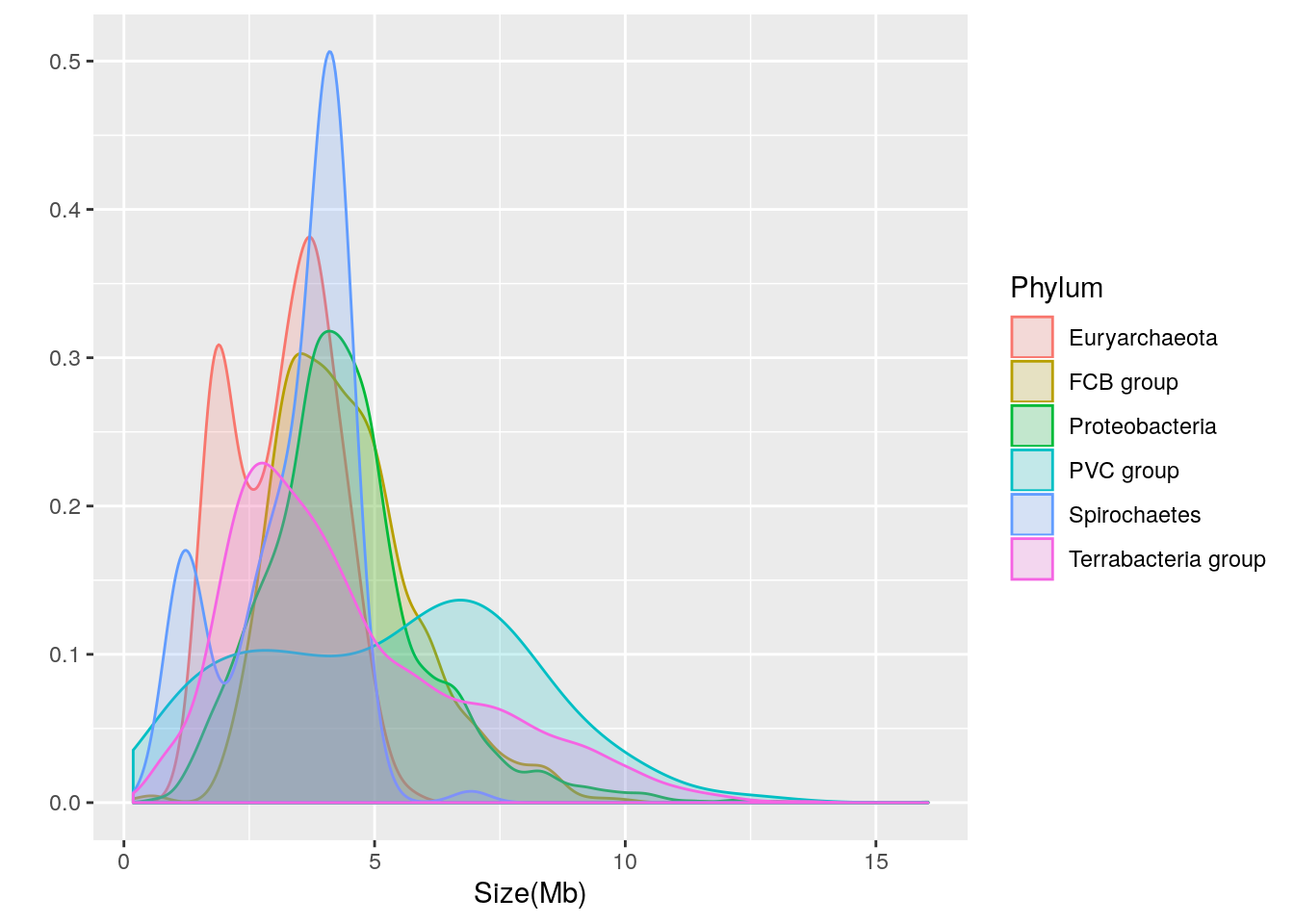
We can see that there is considerable variation in the genome size distribution for each phylum. Let’s get a clearer view by using facets to separate out each phylum:
library(ggplot2)

qplot(data=prokaryote.genomes.table.split.reduced,
      x = `Size(Mb)`,
      geom = "density",
      color = Phylum,
      fill = Phylum,
      facets = Phylum ~ .)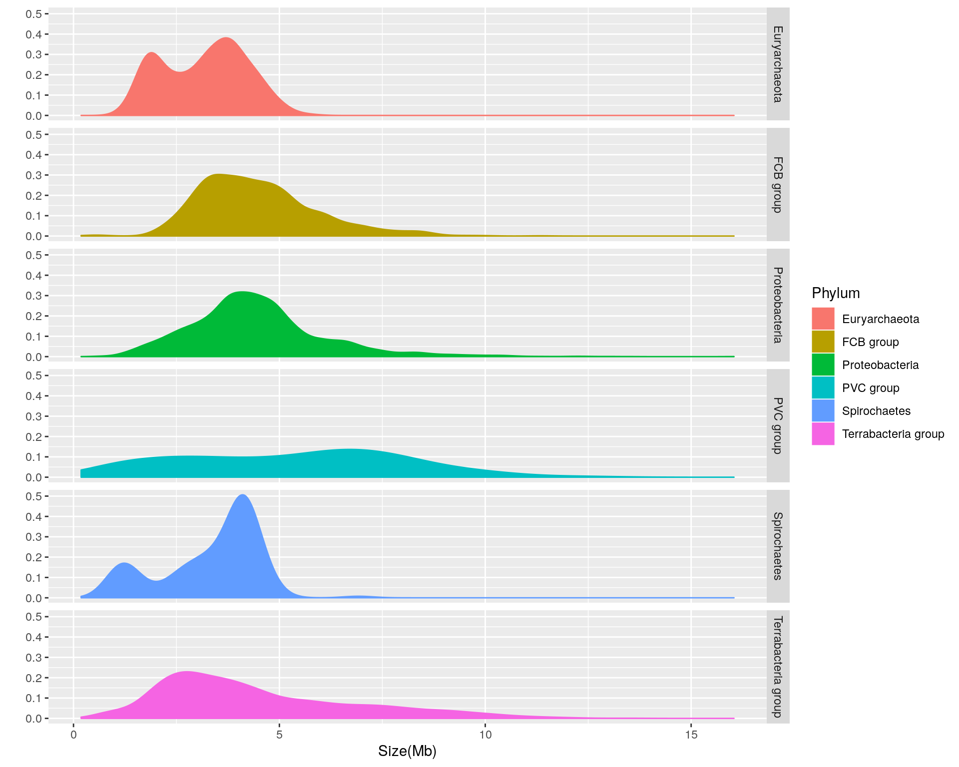
Based upon the separated density plots, it looks as if the genome size varies by phylum. Let’s see how much mean genome size varies by phylum:
- Euryarchaeota = 3.1622121
- FCB group = 4.4686722
- Proteobacteria = 4.4354607
- PVC group = 5.271497
- Spirochaetes = 3.3388135
- Terrabacteria group = 4.4780869
Thus, it appears that phylum-dependent, mean genome size ranges from 3.2 to 5.3 Mb.
Genome Size Positively Correlates with Number of Coding Sequences
The prokaryotic genomes table from NCBI also indicates the number of coding sequences (CDS) in each genome. By creating a scatterplot of genome size vs. CDS, we may examine the relationship between genome size and number of CDS.
library(ggplot2)

qplot(data = prokaryote.genomes.table.split,
      x = `Size(Mb)`,
      y = CDS,
      color = Domain,
      alpha = I(0.2))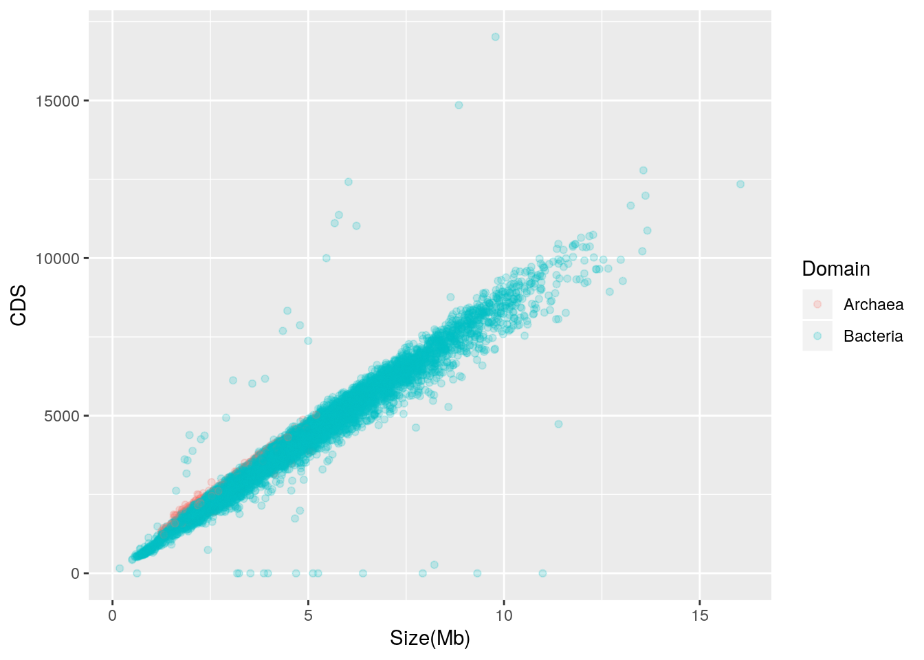
Genome size is strongly and positively correlated with the number of CDS in the genome; put another way, larger genomes have more genes. There are outliers, though, and while those with zero CDS values may be attributable to missing CDS annotation, those with higher than expected CDS should be further explored. Archaea appear to follow a trend similar to Bacteria.
Let’s check to see if the outliers are associated with a single finishing level:
library(ggplot2)
qplot(data = prokaryote.genomes.table.split,
x = `Size(Mb)`,
y = CDS,
color = Level,
alpha = I(0.4))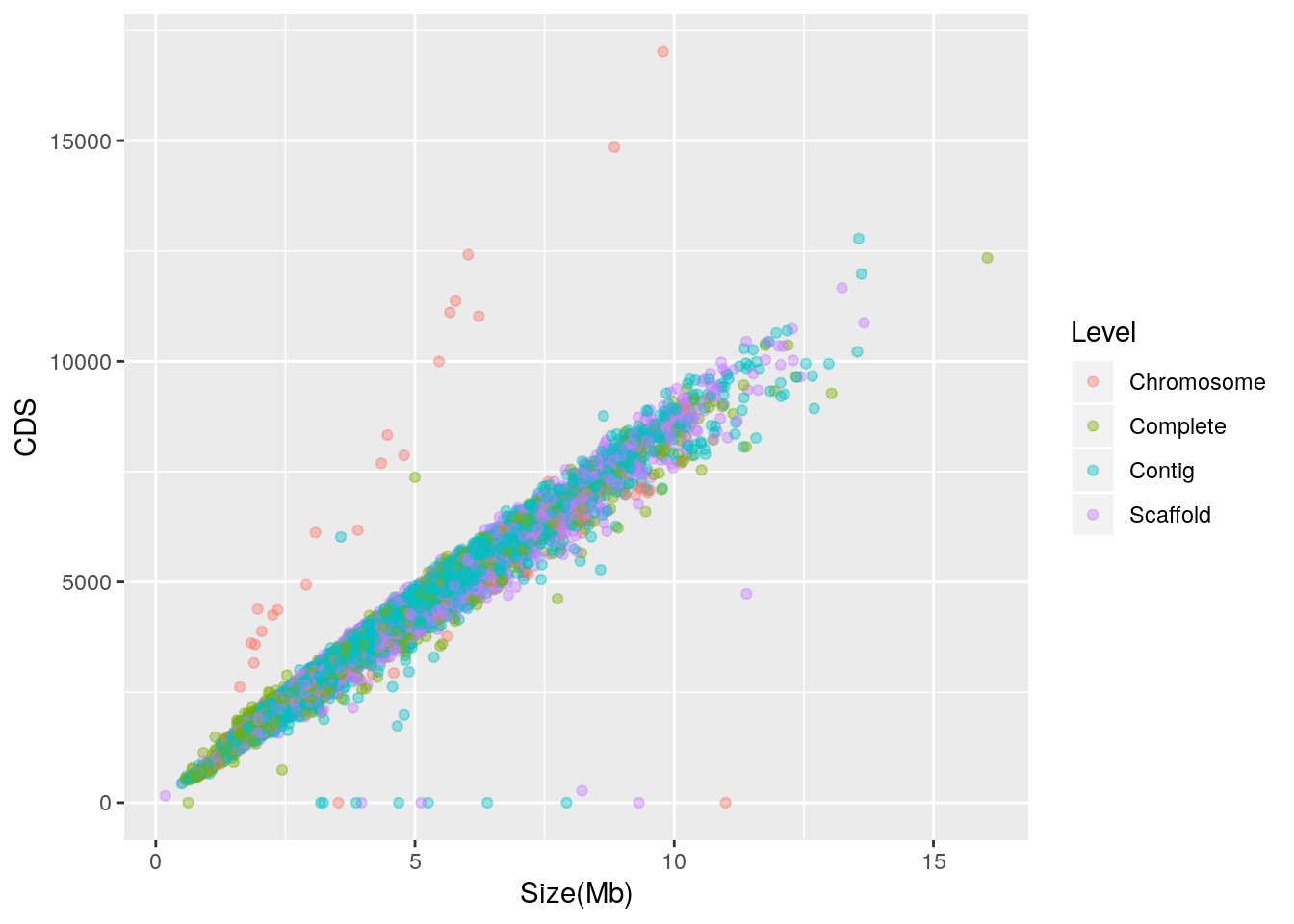 It appears that the outliers with zero CDS are mixed, but most of those with abnormally high CDS for their genome size are labeled as “Chromosome”. In further work, the taxonomic identity of these outliers may be explored.
Conclusion
The genome sizes in this set of 11710 RefSeq representative prokaryotes vary by phylum and span nearly two orders of magnitude from the smallest at 0.185014 Mb to the largest at 16.0407 Mb. The median genome size was determined to be 4.050955 Mb and is a useful approximation that may be used to estimate, for instance, the number of genome equivalents in a given quantity of DNA, or in determining the number of genome equivalents required by a sequencing library preparation, or in determining the number of genome equivalents in the output of a DNA sequencing run.
This webpage was composed using R Markdown, and the Rmd file is available for download and may be viewed as a plain text file or by opening the file within RStudio.